
 Weiguan Wang is a final year PhD student in the Department of Mathematics, under the supervision of Professor Johannes Ruf. His research interests are in machine learning with application to mathematical finance, quantitative finance and fintech.
Following a talk in November 2020 by Professor Johannes Ruf on their joint work, in this blog post Weiguan discusses hedging with machine learning methods. They show that the machine learning methods are able to outperform the traditional method, and justify such an advantage with a well-known financial market fact.
I first came to know financial derivatives in a finance course in my undergraduate in 2010, two years after the 2008 financial crisis. In that course, I learned the usage of derivatives such as options and futures, and the severe consequences they could cause if the risks were not managed well.
Managing the risks, in finance terminology, is called hedging. From now on, we take options as our example for explaining hedging. Assume in the market, we can only buy or sell three assets. They are the stock, the option, and cash. An option gives the holder the right to buy a unit of the stock at a predetermined price in the future, no matter what the future stock price turns out to be. Hence, its price is derived from the stock price, giving the name “financial derivatives”. This price can be derived by a no-arbitrage argument. It says that if two assets have the same cashflow in the future, then its current price must be the same, otherwise there exists an arbitrage. Arbitrage means you can make money for free. In our example, we assume we have sold an option. We can choose some number of the stock to form a portfolio with the option and hold the rest as cash, then this portfolio has value zero today. If tomorrow the total value of the portfolio stays zero regardless of the stock price change, then we say this option is perfectly hedged. The price of the option is just the sum of the cash and what you have spent on buying the stock.
Now let’s work on a simple example. We take a single period binomial tree model. Assume the current stock price is 100, and we sell a option with payoff . The expression means the payoff is the maximum of zero and . Here, is tomorrow’s stock price, and it takes one of the two values with equal probability, given by: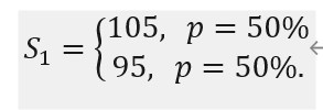
Tomorrow, if the stock price turns out to be 105, the holder of the option can claim £5. Since we sold the option, we need to pay the holder £5. In the other case where the stock price becomes 95, the option expires worthless. Now let’s assume the price of the option is £2.5. Let’s investigate the following portfolio. We borrow £47.5 from the market and buy 0.5 unit of stock (we additionally assume the stock can be split). The £2.5 difference is financed by the sale of the option. This portfolio has zero value, given by 0.5*100-47.5-2.5=0. The positive term indicates a long position, and the negative terms indicate short positions. Tomorrow, the value of the portfolio depends on tomorrow’s stock price, given by:
Now we observe that no matter what the price of the stock turns out to be tomorrow, this portfolio value is always zero, same as its initial value. This option is perfectly hedged with the given portfolio.
The right unit of the stock to hold is called the hedging strategy. The ways to determine it have been investigated for a long time in the financial mathematics community, and this is what I have been working on for my Ph.D. at the LSE, with my supervisor Professor Johannes Ruf.
There have been two streams of hedging. The first approach is traditional and based on modelling the movement of the stock price. A very simple model would be something like the example above; that tomorrow’s stock price will go up or down by 1% with 50% probability each, say. Based on such a model, one can derive the price of the option as a function F of variables including the stock price. Then the hedging strategy is just the partial derivative of the function F with respect to the stock price. This way of hedging is called “Delta hedging”.
However, you wouldn’t believe that the stock price moves like a coin flip, would you? Although there are many more realistic models, they still make strong assumptions on the way the stock price moves in the future. Instead, e propose, along with other researchers, to determine the hedging strategy by means of an artificial neural network (ANN). The ANN is one of the many methods under the scope of machine learning. An ANN is a composition of simple elements called neurons, which maps input features to outputs. Such an ANN then forms a directed, weighted graph; see the following figure. The ANN can be thought of as a statistical model to approximate a function of variables. As we have said, the tradition approach to determine the hedging strategy is calculating the partial derivative of the pricing function F, where the partial derivative is another function of the same set of variables. Hence, the ANN has the potential to approximate the hedging strategy from historical data. To do that, we train the ANN to minimise a quantity called mean squared hedging error. This step is called fitting or optimisation in mathematical terms. This ANN approach leverages the powerful hardware such as graphics processing units (GPUs) and tensor processing units , and it has been proven successful in many applications such as computer vision, language processing, and so on, where a huge amount of data is available. Figure 1. The structure of a two-hidden-layer feed-forward artificial neural network. This ANN has 4 neurons in each hidden layer. More details on the family of ANNs can be found here.
There are two benefits for using ANNs. First, it removes the assumptions on the modelling of the stock movement. The ANN is trained to learn such a movement from historical data directly. Second, the ANN learns the hedging strategy directly, instead of first learning the pricing function and on the second step taking the partial derivative.
We investigate the performance of the ANN on two historical datasets; they are end-of-day data of options written on S&P 500 and tick data of options written on Euro Stoxx 50. Our results yield the same conclusions for both datasets. We show that the ANN can beat the traditional benchmark, i.e. the Nobel Prize winning Black-Scholes model, by about 15%. By interpreting the results, we realise that the ANN can capture a dependency between the stock price and the market volatility (a quantity that measures how volatile the market is), called the leverage effect, while the traditional Black-Scholes model cannot. The leverage effect says that the volatility increases when the stock price decreases. This phenomenon is common in the market, starting from the 1987 Black Monday crash, see Volatility Smile.
Further details on our interpretations of the results can be found in our paper Hedging with Linear Regressions and Neural Networks. You might also be interested in reading our review on this research topic, see Neural Networks for Option Pricing and Hedging: A Literature Review.