 Professor Gregory Sorkin is a Professor in the Operations Research Group in the LSE Department of Mathematics, working on discrete random systems and optimisation. This blog post is an abridged version of an article he wrote that was accepted to The Mathematical Intelligencer; the extended article can be found here.
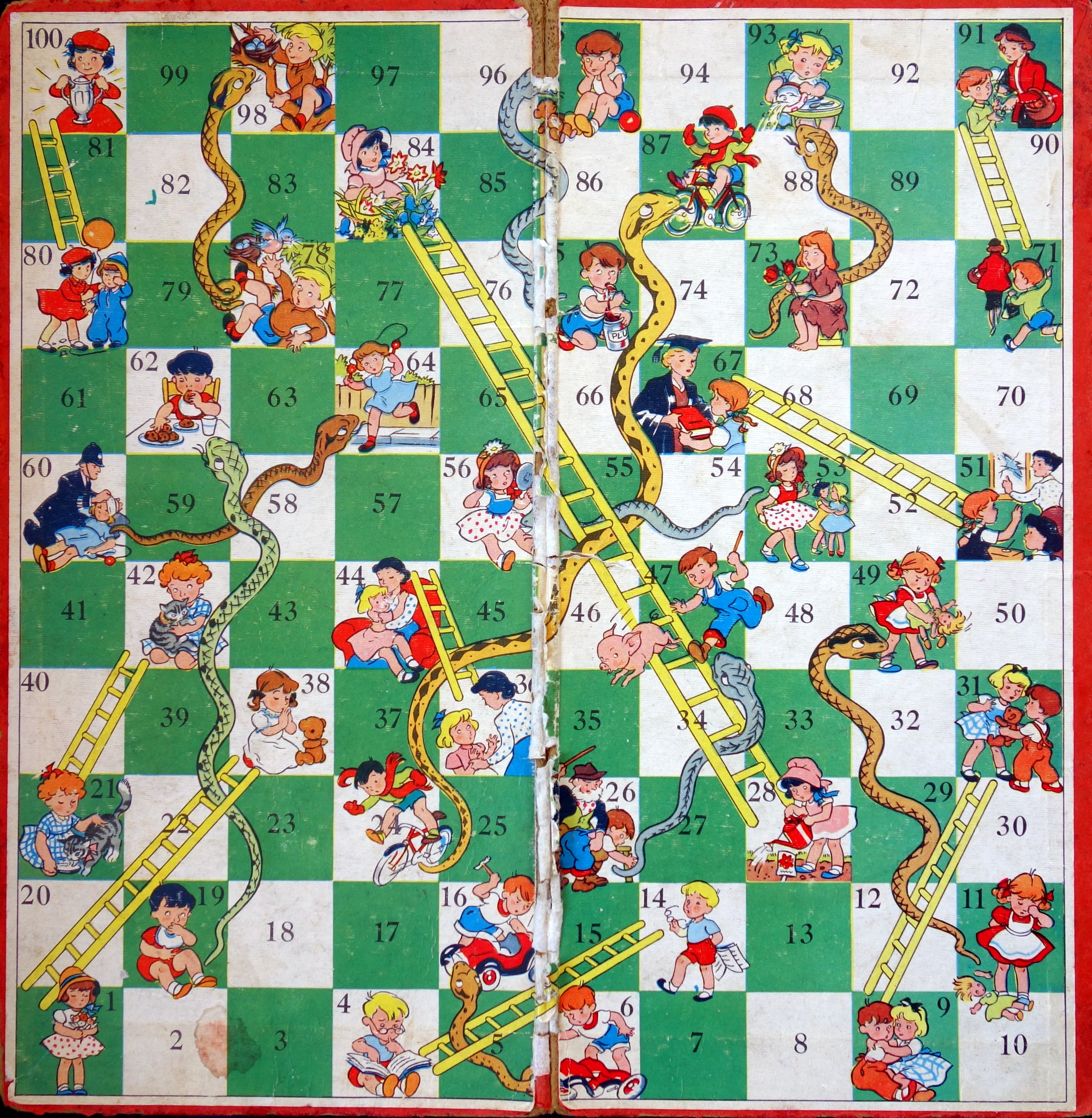
For those fortunate enough to be unfamiliar with it, Snakes and Ladders is a children’s board game of no skill and no mathematical interest. There is a board that is in essence a strip of squares, from 1 to 100. A sample board is shown in Figure 1. Each player starts in square 0 (just off the board), and players take turns. On each turn, a player rolls a standard 6-sided die, and advances by a number of squares equal to the roll of the die. The twist is that some squares (“ladders”), when you land on them, advance you to a later square, and some (“snakes”) put you back to an earlier square. The goal is to be first to reach square 100. If you “overshoot” the target square 100, you reflect back; so from 99, a roll of 3 would bring you 1 step forward to 100, then 2 steps back to 98… where on our board there is a snake, so you’d wind up at 78.
A key point is that the players are independent. They could as well play separately, each counting how many moves they took, and compare notes at the end: the one with the smaller number of moves wins. This, and the fact that no skill is involved (there are no choices to make), are why I disparaged the game as being of no (mathematical) interest, but actually there are interesting aspects.
In particular, as the game is played, both players tend to advance, but there are frequent setbacks. When you are at square i and your opponent is at j, it is natural to wonder who has the advantage. We’ll say that square i is “better than” j (and write “i > j”) if i is more likely to win than j is: if the two players bet even odds on the outcome, in the long run i would win. Are later squares always better? Probably not, as it’s probably better to have the possibility of a long ladder just ahead of you than to be just past it. Does it even make sense to ask what square is better, or does it depend on your opponent’s square? Specifically, might the game be “intransitive”: is it possible that square i is better than j, and j better than k, but k better than i, so that i > j > k > i?
We will answer these questions. We are not aware of the intransitivity question having been asked before for Snakes and Ladders. Along the way, we’ll visit Markov chains, simulation, a paradox of size-biased sampling (but not in this abridged version), and intransitive dice.
First, a soupçon of history and some details.
History, details, and the Markov chain
Snakes and Ladders is widely agreed to derive from an Indian game, called gyān chaupar in Hindi, making its way to Victorian England as a side effect of British colonialism. An item on the Snakes and Ladders Wikipedia page asserts without attribution that the game has been played since the 2nd century AD, while a number of sources credit its origin to the 13th century Sant Dnyaneshwar, but again without citing any basis. A scholarly article [1] cites concrete evidence for the game’s play in the 18th century and says it “is doubtless much older”, but that since the board materials are ephemeral, “[u]ntil earlier evidence is available, the origins … of the game must remain obscure.” The boards vary in size, the number of snakes and ladders, and their positions, depiction, and labelling, but the game play remains the same. On both continents, the game was meant to be morally educational. Virtuous ladders, and vices represented by snakes, would bring you towards or away from some version of heaven. Their depiction and labelling would suit the morality of the time and place; a Victorian version, for example, having a ladder of Penitence leading to a square of Grace.
Whether or not morally instructive, the game is a fine illustration of randomness.
Let’s return to the game’s setup and clarify some details. First, an example. In our board, there is a ladder from square 4 to 14. This means that square 4 can never be occupied: if for example a player is on square 3 and rolls a 1, they move to square 14.
| 38 | 2 | 3 | 14 | 5 | 6 | 7 | 8 | 31 | 10 |
| 11 | 12 | 13 | 14 | 15 | 6 | 17 | 18 | 19 | 20 |
| 42 | 22 | 23 | 24 | 25 | 26 | 27 | 84 | 29 | 30 |
| 31 | 32 | 33 | 34 | 35 | 44 | 37 | 38 | 39 | 40 |
| 41 | 42 | 43 | 44 | 45 | 46 | 26 | 48 | 11 | 50 |
| 67 | 52 | 53 | 54 | 55 | 53 | 57 | 58 | 59 | 60 |
| 61 | 19 | 63 | 60 | 65 | 66 | 67 | 68 | 69 | 70 |
| 91 | 72 | 73 | 74 | 75 | 76 | 77 | 78 | 79 | 100 |
| 81 | 82 | 83 | 84 | 85 | 86 | 24 | 88 | 89 | 90 |
| 91 | 92 | 73 | 94 | 75 | 96 | 97 | 78 | 99 | 100 |
| 99 | 78 | 97 | 96 | 75 |
Figure 2. Our Snakes & Ladders board, shown here laid out from top to bottom and left to right, not bottom to top in a serpentine pattern as conventional. The first entry is 38 because square 1 has a ladder to 38, squares 2 and 3 are straightforward, square 4 has a ladder from 4 to 14, and so forth. Square 95 is replaced by a snake to 75, and the finishing square of 100 is followed by the squares to which you are redirected if you overshoot 100.
An important detail is what it means to win. One definition is that if you are the first to finish, you win (a Markov chain analysis of this version of the game is given in [Aud12]). But this gives an advantage to the first player. In our house we play fair: the game goes in rounds (player 1, then player 2), and a player wins if they finish in a round and the other player does not. So, if player 1 finishes, player 2 has one last roll of the dice: if they also finish, the game is a draw.
Here’s why we care here. We’re looking for “intransitivity”, namely a cycle, specifically a triangle, where square i is better than j, j is better than k, and k is better than i. When we say i > j, we mean that if we are in square i and our opponent is in j, we have a winning edge: we win more than they do (with draws not counting either way). But with the “unfair” rules, and assuming it is my turn next, i > i : if both players are in square i, clearly I have an advantage. This leads to a trivial, uninteresting cycle of advantage.
So, our definition here is that the player finishing in an earlier round wins, and if both finish in the same round it is a draw.
To recapitulate, in essence, the game consists of a set of squares or “states”. From each state, there are 6 possible next states, the actual one depending on the roll of the die. This defines a Markov chain (see Figure 2). Our board has 84 states including 0 and 100: squares that are the starting point of a snake or ladder do not appear as states since it is impossible to wind up in such a square. The winner is the first player to reach a specified state (100, in our case).
Expected time to finish
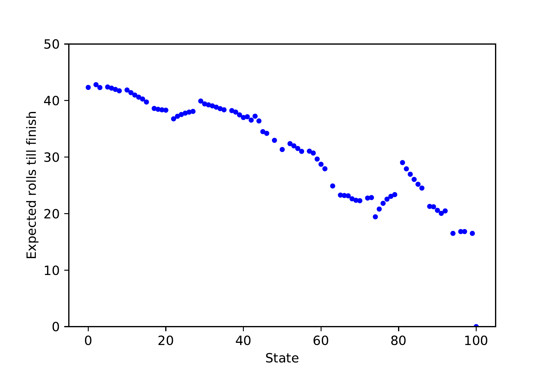
Let’s return now to our questions. It’s natural to wonder, first, to what degree being further along the board is actually helpful, and by how much. For each state (each board square that is not the start of a snake or ladder), what is the expected number of moves until finishing: the number of moves it would take, on average, over an infinite number of games?
Figure 3 shows that indeed it is generally better to be further advanced along the board — later squares have a lower expected time to completion — but there are many exceptions. For instance, the situation is successively worse from squares 22 to 27, because square 28 is a ladder to 84, and being a bit earlier maximises the chance of landing at that ladder.
The results shown here are drawn from more detailed results giving, for each state i, the probability that, starting in state i, the game finishes within k moves; in principle this should be done for all k from 0 through ∞, but in practice, the chance the game has not ended after 1,000 moves is less than 10 − 14 (even for the worst-case starting square) so we limited calculation to this. This is equivalent to knowing, for each k, the probability that the game ends precisely on the kth roll: the differences in successive “by time k” probabilities are the “at time k” ones, and the cumulative sums of the “at k” probabilities are the “by k” ones. There are two methods of going about finding this information: simulation of the game, or calculation from the Markov transition matrix.
Simulation
Since these questions were just a flicker of curiosity, not a serious research agenda, it was natural to address them by a quick and easy simulation. We can program a computer to start a player in a specified square i, perform a simulated die roll, advance the player accordingly, and stop when the player finishes. Repeating this for square i gives a sample of the game lengths that, with a large number of repetitions, should be an accurate sample of the true distribution of the duration.
Observing that the game is memoryless, the simulation can be done much more efficiently. Memorylessness means that, if we are in square i, the remaining time until the end of the game is independent of what came earlier (though of course random depending on the future die rolls). Thus, instead of getting just a single duration out of one game simulation, we can get many. Suppose a simulated game visits squares 0, 2, 6, 10, 6, 9, …, 100, with 50 steps after the 0. (From square 10, a roll of 6 brings you to square 6 via a ladder at 16.) This play gives 51 simulated values: from 0 the game ended in 50 steps, from 2 in 49 steps, and so on, until from 100 it ended in 0 steps. Note that from the first 6 the game ends in 48 steps, and from the second 6 in 46 steps: the simulation can give several remaining-time samples for a single i. All in all, a play of n steps gives n samples (ignoring the final 100), much better than playing a whole game to get just one sample.
Markov chain
The Snakes and Ladders Markov chain, like any other, is completely described by its transition matrix A. For states i and j, Aij is the probability of moving from state i to state j in one step. Here, for example, A17, 19 = 1/6: a die roll of 2 (only) brings us from 17 to 19. To get from i to j in exactly two steps means moving from i to some k in one step and k to j in the next, which happens with probability ∑k AikAjk = (A2)ij. Repeating this gives a fundamental property of Markov processes, that the probability of getting from i to j in exactly s steps is (As)ij.
If we are interested in the probability, starting from i, of reaching the final state 100 in s steps, here that is given by (As)i, 100. Specifically, the finishing state is “absorbing”: from state 100 there is probability 1 of returning to 100 (A100, 100 = 1) and probability 0 of moving to any other state. In this case (As)i, 100 represents the probability of being in the finish state at time s (perhaps having reached the state earlier). As remarked earlier, (As)i, 100 − (As − 1)i, 100 is the probability that the game duration, from i, is exactly s.
So, repeating for say s from 0 to 1, 000 gives the probability (As)i, 100 that, for each start state i, the game ends at time s. In practice, this gives, for each i, the distribution of game lengths (the only error being the < 10 − 14 fraction of games that are longer than 1, 000 rolls).
Let’s quickly return to the expected game durations from each state. Let fi(s) be the probability that the game, starting from i, ends in exactly s steps. Then, the expected duration of the game, from i, is simply ∑s ≥ 0 sfi(s). This leads to the results shown in Figure 3.
Pair competitions and intransitivity
What about the probability that a player in state i finishes in fewer rounds than an opponent in state j? For any state i, define gi(s) = ∑t ≤ s fi(s); this is the probability that the game has finished within time s, starting from i. For i to beat j means that i finishes in some round s by which j has not yet finished, so i beats j with probability
Qij := ∑s ≥ 0 fi(s)(1 − gj(s)).
Truncating this to a finite sum gives our estimate of the probability Qij that i beats j. We compute this for all pairs i, j. Specifically, for each s we compute the array of all fi(s)(1 − gj(s)) values. This calculation is perhaps not as elegant as could be, but it is efficient enough.
Define the “excess” Xij of i over j by Xij = Qij − Qji, the win probability of i over j versus that of j over i. If on each game the winner got £1, with no money exchanged for a draw, Xij would be i’s average winning, playing against j. We won’t need it, but the probability of a draw is just 1 − Qij − Qji.
Our original question translates to whether there are states i, j, k such that Xij, Xjk, and Xki are all positive. Specifically, let’s look for such states where Xij ≥ c, Xjk ≥ c, and Xki ≥ c, and c is as large as possible.
The result is that states 69, 79, and 73 form such a triangle, each with a winning edge at least 1/2% over the next in the cycle. Specifically, state 69 has a winning edge over state 79 of X69, 79 ≈ 0.0077, with larger wins of X79, 73 ≈ 0.0112 and X73, 69 ≈ 0.0171. The respective win probabilities are Q69, 79 ≈ 0.4970, Q79, 73 ≈ 0.4990 and Q73, 69 ≈ 0.4930.
Checking by simulation
These figures were checked against simulations. Starting from 0, 100, 000 games were simulated, with a total of about 4.4M die rolls; the maximum game length observed was under 500 rolls. Each of the three states in question was visited at least 25,000 times. Comparing with the calculated winning edges above, namely 0.0077, 0.0112, and 0.0171, the simulated ones were about 0.0090, 0.0096, and 0.0172. A second simulation gave similar results: 0.0081, 0.0127, 0.0146. Each simulation’s time is dominated by the gameplay, taking under 3 minutes in an inefficient implementation. Simulations with 10,000 games are even less accurate, often showing negative values rather than the positive ones desired. A simulation with 1M games takes 5 minutes (in a quickly improved implementation) and gives results wonderfully close to the calculated ones: 0.0072, 0.0115, and 0.0171 (each off by at most 0.0005 from the calculation).
Intransitive dice
Despite having been open to the theoretical possibility of there being intransitivity in Snakes and Ladders, I was struck by this result. I did not know anything else like it. I expected that something related must be known and did an Internet search but, not knowing the right keywords, did not quickly find anything. I reached out to a couple of colleagues and got an almost immediate response from Bernhard von Stengel: “intransitive dice”. I will not attempt to summarise the literature, but there is (as usual) a nice Wikipedia article.
One example taken from the article is three six-sided dice, die A labelled 2, 2, 6, 6, 7, 7, B labelled 1, 1, 5, 5, 9, 9, and C labelled 3, 3, 4, 4, 8, 8. Aside from the conventionality and physical practicality of six sides, we can as well think of these as three-sided dice, die A labelled 2, 6, 7, B labelled 1, 5, 9, and C labelled 3, 4, 8. Note that there are no ties. Die A beats B 5/9ths of the time, for an edge of 1/9th, where here winning means having a larger value.
The full version of the present article finds a set of three dice that are in some sense minimal. This prompted a referee to ask for a minimal intransitive snakes and ladders board, and here we leave this as a puzzle for the reader.
[1] Andrew Topsfield. The indian game of snakes and ladders. Artibus Asiae, 46(3):203-226, 1985.
[2] Daniel Audet. Probabilités et espérances dans le jeu de serpents et échelles à deux joueurs. Bulletin AMQ, LII(4), Dec 2012.