 The weight placed on p-values and significance testing has come under increasing criticism, with one social psychology journal banning their use entirely. Nicole Radziwill argues that many of the issues come down to sampling errors. Inferential statistics is good because it lets us make decisions about a whole population based on one sample. But inferential statistics is bad if your sample size is too small. Using the statistical programming language R and data on grade point averages, she demonstrates just how easy it can be to accidentally draw wrong conclusions and what can be done to fix this.
Just recently, the editors of the academic journal Basic and Applied Social Psychology have decided to ban p-values: that’s right, the nexus for inferential decision making… gone! This has created quite a fuss among anyone who relies on significance testing and p-values to do research (especially those, presumably, in social psychology who were hoping to submit a paper to that journal any time soon). The Royal Statistical Society even shared six interesting letters from academics to see how they felt about the decision.
These letters all tell a similar story: yes, p-values can be mis-used and mis-interpreted, and we need to be more careful about how we plan for — and interpret the results of — just one study! But not everyone advocated throwing out the method in its entirety. I think a lot of the issues could be avoided if people had a better gut sense of what sampling error is… and how easy it is to encounter (and as a result, how easy it can be to accidentally draw a wrong conclusion in an inference study just based on sampling error). I wanted to do a simulation study to illustrate this for my students.
The Problem
You’re a student at a university in a class full of other students. I tell you to go out and randomly sample 100 students, asking them what their cumulative Grade Point Average (GPA) is. You come back to me with 100 different values, and some mean value that represents the average of all the GPAs you went out and collected. You can also find the standard deviation of all the values in your sample of 100. Everyone has their own unique sample.
“It is misleading to emphasize the statistically significant findings of any single team. What matters is the totality of the evidence.” – John P. A. Ioannidis in Why Most Published Research Findings are False
It’s pretty intuitive that everyone will come back with a different sample… and thus everyone will have a different point estimate of the average GPA that students have at your university. But, according to the central limit theorem, we also know that if we take the collection of all the average GPAs and plot a histogram, it will be normally distributed with a peak around the real average GPA. Some students’ estimates will be really close to the real average GPA. Some students’ estimates will be much lower (for example, if you collected the data at a meeting for students who are on academic probation). Some students’ estimates will be much higher (for example, if you collected the data at a meeting for honors students). This is sampling error, which can lead to incorrect inferences during significance testing.
Inferential statistics is good because it lets us make decisions about a whole population just based on one sample. It would require a lot of time, or a lot of effort, to go out and collect a whole bunch of samples. Inferential statistics is bad if your sample size is too small (and thus you haven’t captured the variability in the population within your sample) or have one of these unfortunate too-high or too-low samples, because you can make incorrect inferences. Like this.
The Input Distribution
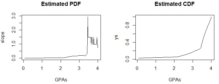
Let’s test this using simulation in R. Since we want to randomly sample the cumulative GPAs of students, let’s choose a distribution that reasonably reflects the distribution of all GPAs at a university. To do this, I searched the web to see if I could find data that might help me get this distribution. I found some data from the University of Colorado Boulder that describes GPAs and their corresponding percentile ranks. From this data, I could put together an empirical cumulative distribution function (CDF), and then since the CDF is the integral part of the probability density function (PDF), I approximated the PDF by taking the derivatives of the CDF. (I know this isn’t the most efficient way to do it, but I wanted to see both plots):
score <- c(.06,2.17,2.46,2.67,2.86,3.01,3.17,3.34,3.43,3.45,
3.46,3.48,3.5,3.52,3.54,3.56,3.58,3.6,3.62,3.65,3.67,3.69,
3.71,3.74,3.77,3.79,3.82,3.85,3.88,3.91,3.94,3.96,4.0,4.0)
perc.ranks <- c(0,10,20,30,40,50,60,70,75,76,77,78,79,80,81,
82,83,84,85,86,87,88,89,90,91,92,93,94,95,96,97,98,99,100)
fn <- ecdf(perc.ranks)
xs <- score
ys <- fn(perc.ranks)
slope <- rep(NA,length(xs))
for (i in 2:length(xs)) {
 slope[i] <- (ys[i]-ys[i-1])/(xs[i]-xs[i-1])
}
slope[1] <- 0
slope[length(xs)] <- slope[length(xs)-1]
Then, I plotted them both together:
par(mfrow=c(1,2))
plot(xs,slope,type="l",main="Estimated PDF")
plot(xs,ys,type="l",main="Estimated CDF")
dev.off()
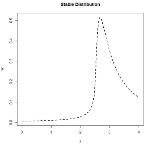
I looked around for a distribution that might approximate what I saw. (Yes, I am eyeballing.) I found the Stable Distribution, and then played around with the parameters until I plotted something that looked like the empirical PDF from the Boulder data:
x <- seq(0,4,length=100)
hx <- dstable(x, alpha=0.5, beta=0.75, gamma=1, delta=3.2)
plot(x,hx,type="l",lty=2,lwd=2)
The Simulation
First, I used pwr.t.test to do a power analysis to see what sample size I needed to obtain a power of 0.8, assuming a small but not tiny effect size, at a level of significance of 0.05. It told me I needed at least 89. So I’ll tell my students to each collect a sample of 100 other students.
Now that I have a distribution to sample from, I can pretend like I’m sending 10,000 students out to collect a sample of 100 students’ cumulative GPAs. I want each of my 10,000 students to run a one-sample t-test to evaluate the null hypothesis that the real cumulative GPA is 3.0 against the alternative hypothesis that the actual cumulative GPA is greater than 3.0. (Fortunately, R makes it easy for me to pretend I have all these students.)
sample.size <- 100
numtrials <- 10000
p.vals <- rep(NA,numtrials)
gpa.means <- rep(NA,numtrials)
compare.to <- 3.00
for (j in 1:numtrials) {
     r <- rstable(n=1000,alpha=0.5,beta=0.75,gamma=1,delta=3.2)
     meets.conds <- r[r>0 & r<4.001]
     my.sample <- round(meets.conds[1:sample.size],3)
     gpa.means[j] <- round(mean(my.sample),3)
     p.vals[j] <- t.test(my.sample,mu=compare.to,alternative="greater")$p.value
     if (p.vals[j] < 0.02) {
          # capture the last one of these data sets to look at later
     capture <- my.sample
     }
}
For all of my 10,000 students’ significance tests, look at the spread of p-values! They are all over the place! And there are 46 students whose p-values were less than 0.05… and they rejected the null. One of the distributions of observed GPAs for a student who would have rejected the null is shown below, and it looks just fine (right?) Even though the bulk of the P-Values are well over 0.05, and would have led to the accurate inference that you can’t reject the null in this case, there are still plenty of values that DO fall below that 0.05 threshold.
> summary(p.vals)
 Min. 1st Qu. Median Mean 3rd Qu. Max.
0.005457 0.681300 0.870900 0.786200 0.959300 1.000000
> p.vals.under.pointohfive <- p.vals[p.vals<0.05]
> length(p.vals.under.pointohfive)
[1] 46
> par(mfrow=c(1,2))
> hist(capture,main="One Rogue Sample",col="purple")
> boxplot(p.vals,main="All P-Values")
Even though the p-value shouted “reject the null!” from this rogue sample, a 99% confidence interval shows that the value I’m testing against… that average cumulative GPA of 3.0… is still contained within the confidence interval. So I really shouldn’t have ruled it out:
> mean(capture) + c(-1*qt(0.995,df=(sample.size-1))*(sd(capture)/sqrt(sample.size)),
+ qt(0.995,df=(sample.size-1))*(sd(capture)/sqrt(sample.size)))
[1] 2.989259 3.218201
> t.test(capture,mu=compare.to,alternative="greater")$p.value
[1] 0.009615011
If you’re doing real research, how likely are you to replicate your study so that you know if this happened to you? Not very likely at all, especially if collecting more data is costly (in terms of money or effort). Replication would alleviate the issues that can arise due to the inevitable sampling error… it’s just that we don’t typically do it ourselves, and we don’t make it easy for others to do it. Hence the p-value controversy.
What Now?
What can we do to improve the quality of our research so that we avoid the pitfalls associated with null hypothesis testing completely, or, to make sure that we’re using p-values more appropriately?
- Make sure your sample size is big enough. This usually involves deciding what you want the power of the test to be, given a certain effect size that you’re trying to detect. A power of 0.80 means you’ll have an 80% chance of detecting an effect that’s actually there. However, knowing what your effect size is prior to your research can be difficult (if not impossible).
- Be aware of biases that can be introduced by not having a random enough or representative enough sample.
- Estimation. In our example above we might ask “How much greater than 3.0 is the average cumulative GPA at our university?” Check out Geoff Cummings’ article entitled “The New Statistics: Why and How” for a roadmap that will help you think more in terms of estimation (using effect sizes, confidence intervals, and meta-analysis).
- Support open science. Make it easy for others to replicate your study. If you’re a journal reviewer, consider accepting more articles that replicate other studies, even if they aren’t “novel enough”.
I am certain that my argument has holes, but it seems to be a good example for students to better embrace the notion of sampling error (and become scared of it… or at least more mindful). Please feel free to suggest alternatives that could make this a more informative example. Thank you!
This piece originally appeared on the author’s personal blog Quality and Innovation and is reposted with permission.
Featured Image credit: systematic sampling technique by Dan Kernler (Wikimedia, CC BY-SA 4.0)
Note: This article gives the views of the author, and not the position of the Impact of Social Science blog, nor of the London School of Economics. Please review our Comments Policy if you have any concerns on posting a comment below.
Nicole Radziwill is an Associate Professor (as of Fall 2015) in the Department of Integrated Science and Technology at James Madison University (JMU), where she has been on the faculty since 2009. Nicole is also a Fellow of the American Society for Quality (ASQ), Certified by ASQ as a Manager of Quality and Organizational Excellence (CMQ/OE), and an ASQ Certified Six Sigma Black Belt (CSSBB). She was Chair of the ASQ Software Division from 2009 to 2011, a national Examiner for the Malcolm Baldrige National Quality Award (MBNQA) in 2009 and 2010, and has a PhD in Technology Management and Quality Systems from Indiana State University. She also has an MBA and a BS degree in Meteorology from Penn State. Nicole was recognized by Quality Progress in 2011 as one of the 40 New Voices of Quality, and serves as one of ASQ’s Influential Voices bloggers.


A nitpick, but perhaps an important point: collecting your data at a meeting of students on probation is not sampling error, but systematic error.
Hi Brendan – indeed, very good point and many thanks for the clarification. However, if you aren’t *aware* that your sample is not representative, the systematic error will look just like sampling error.
Dear Nicole Radziwill,
Your simulation is wrong for many reasons to address your goal!! Most importantly your sample in each run is neither independent nor identical. Check CLT on Wikipedia!