Felix Brown, BSc. PPE ’25 (Reading time 10 minutes)
T-tests, ANOVA, p-values, confidence intervals. If you have read political science papers before I am sure that you have encountered these techniques being used to compare theories and observed data. However, they are not the only way to approach quantitative research in political science, representing only one of two possible statistical paradigms: Frequentism and Bayesianism. Frequentism is currently the dominant paradigm but Bayesian methods and thinking are increasingly gaining popularity in political science. This guide explains what these two paradigms are, providing examples of both in practice. It also explains the benefits of using Bayesian methods in political science and how it overcomes some frequentist shortcomings.
Main takeaways
- The accurate interpretation of frequentist sample statistics
- Frequentist techniques like t-tests and confidence intervals are not appropriate for answering some political science questions
- The different components of Bayesian Inference
- The benefits of Bayesian Inference
Understanding Frequentist Probability
Frequentists see probability as representing the objective long run frequency of an event.
For example, if I flipped a coin, frequentists argue that if I did so infinitely many times, the objective probability of a coin flip resulting in heads could be learned. However, since infinite repetitions is in reality impossible, it is more realistic to have a limited sample of say 1 million coin flips. To answer the question of the probability of heads a coin flip resulting in heads, a frequentist would compute a 95% confidence interval using the sample, an example of which is below.
95% CI[0.4999,0.50101]
Often, even in political science papers, such a result is interpreted as meaning that the objective probability of heads lies in the confidence interval with 95% probability. This is a misunderstanding of what can be inferred from the statistic. The confidence interval instead relates to the reliability of the estimation procedure; all that can be inferred is that if the procedure of sampling 1 million coin flips were repeated, yielding different samples, approximately 95% of calculated confidence intervals would contain the true probability of getting heads (Pr(heads)). This same unintuitive logic underpins aforementioned techniques like t-tests and p-values. Although this can be conceptually confusing without having studied statistics, the main takeaway of this clarification should be that frequentist statistics relies on the theoretical possibility of repeated sampling to be meaningful.
Although repeated sampling and therefore frequentist statistics make sense in the context of a coin flip, when the frequentist interpretation of probability is applied to many questions in political science, it becomes nonsensical. What if, like Jackon 2004, you were a political scientist predicting the distribution of votes in Florida before the 2000 US presidential election and there was a recently released poll of Florida voters. Under a frequentist paradigm, common practice is to use a confidence interval to make inferences from the data.
95% CI[50.7%, 59.3%] (republic share of the vote, excluding third party voters)
The correct interpretation of this confidence interval is that if a sample of Florida voters were collected using the same sampling technique of the poll, the resulting confidence intervals would constrain the population republican vote share 95% of the time. Direct claims about the outcome of the election cannot be made. Consequently, frequentist reference to repeated sampling and long run frequency is insufficient to answer some questions in political science. However, there is an alternative paradigm to frequentism for understanding probability and statistics: Bayesianism
Explaining Bayesian Inference
Foundations
Bayesianism stems from an alternative understanding of the meaning of probability to frequentism. Instead of representing a natural characteristic of a population that can be discovered through repeated trials, probability represents rational degrees of belief in a proposition given available information. Returning to the coin toss example, a Bayesian interpretation of the value assigned to Pr(heads) is the individual’s confidence the coin toss’ resulting in heads, taking into account all relevant, available information such as if the coin is biassed. There are multiple useful implications of this alternative Bayesian understanding of probability for answering questions in political science using data, notably allowing direct claims beyond repeated sampling and contextualising new information, which I will expand on following an explanation of the process.
Bayes’ Formula
The engine of Bayesian Inference is Bayes’ Formula.
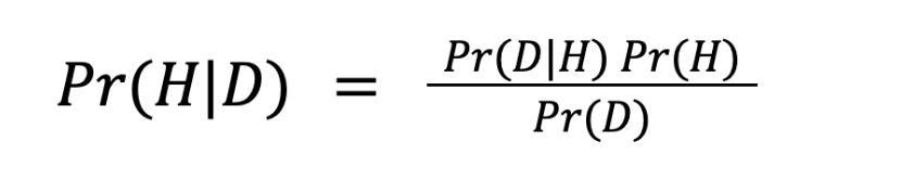
Pr(x) denotes rational degrees of belief in proposition x
Pr(x|y) denotes conditional probability of x given y
H denotes a proposition
D denotes new information/data to be incorporated
If you have taken an introductory probability and statistics course, it is very likely you have encountered the formula in its general form and used it to calculate conditional probabilities. Although the underlying intuition is the same in this context, the formula’s components denote specific meanings.
Priors
On the RHS of the formula is term Pr(H), referred to as the “prior”. The use of priors are central to the divergence between frequentist and Bayesian inference. Priors denotes the probability, meaning degree of confidence, in the proposition without knowledge of information D. Hence, priors are determined by relevant background information.
Likelihood
The conditional probability of the data being observed assuming the hypothesis is true is called the likelihood and is denoted by Pr(D|H). Likelihoods capture the intuition that observed data that fits well with H means more confidence should be had in H, leading to a higher posterior.
Probability of the Data
P(D) refers to the degree of confidence in the observed data set. The intuition behind this is that when making inferences from data with respect to a conclusion, the extent to which we believe the data to be accurate should shift the confidence we have in that inference. However, this component is sometimes left out.
Posterior
Substituting probabilities or probability distributions into the components of the RHS of Bayes’ formula yields P(H|D), known as the posterior. The posterior reflects an updating of prior beliefs concerning H given new information D.
Hence, on the intuitive level, Bayesian Inference formalises the process of incorporating new information into our belief about a proposition. It demonstrates that when new data is acquired, the degree of confidence in the data, the likelihood of observing the data if the proposition was true and our prior confidence in the proposition inform our updated confidence in the proposition.
An important note for engaging with Bayesian analysis is the above explination’s use of the simplifying assumption that the components of Bayes’ formula refer to probabilities. In quantitative analysis, they generally instead refer to probability distributions, giving information about the shape of the data and our confidence in it, not just a point estimate.
Bayesian Credible Intervals
*note this section is more mathematical
Given an understanding of the components of Bayesian Inference, it is possible to create a Bayesian equivalent to the frequentist confidence interval, referred to as a credible interval, of Simon Jackman’s example of predicting the outcome of Florida in the 2000 Bush-Gore US presidential election. The technique is structured around Bayes’ Formula, meaning I will explain the formula’s components in the context of predicting the 2000 presidential election given new polling data.
Pr(Bush’s % of the vote in Florida|Polling Data) =
Pr(Polling data |Bush’s % of the vote in Florida) Pr(Bush’s % of the vote in Florida)
Priors
Since priors represent belief in Bush’s vote share before incorporating the polling data, they are derived from any relevant, available information. Although more complex priors with multiple sources of information could be used, for the sake of simplicity, this model’s priors will be based on data on the republican vote share in Florida during previous presidential elections.
Using state-level presidential election outcomes from 1932-1996, Jackson creates a regression model with fixed effects for every state and year, with republican % of the vote as the outcome. In this context, fixed effects means the regression individually calculates the effect of being each state and being each year on the outcome. A prediction for Florida’s republican % was then calculated through averaging the fixed effect for Florida and the median fixed effect for year, resulting in a prediction of 49.1% with a standard error of 2.2%. To allow for Bayesian Inference, it is then assumed that the regression prediction can be characterised with a normal distribution, meaning the prior is:
Pr(Bush’s % of the vote in Florida) ~ N(49.1, 2.2 )
Likelihood
Jackson also assumes the polling data is normally distributed. Hence, using the sample average and standard deviation, the likelihood is given by the polling data.
Pr(Polling Data|Bush’s % of the vote in Florida) ~ N(55, 2.2 )
Posterior
Since the likelihood and prior distributions are both known, the posterior distribution can be calculated by combining the two. In this case Pr(Polling Data) can be ignored. I will not go into how the two probability distributions are combined to avoid mathematical complexity but combining them yields a third normal distribution with mean 52.1 and standard deviation 1.6.
Pr(Bush’s % of the vote in Florida|Polling Data) ~ N(52.1, 1.6)
Finally, a 95% credible interval can be calculated using the mean and standard deviation of the posterior distribution.
Bush’s % of the vote in Florida 95% CI[48.9%, 55.2%]
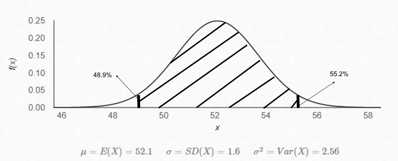
The posterior distribution and its 95% credible interval can also be represented graphically, where the shaded area is where Bush’s % should be 95% of the time.
Returning to the Frequentist-Bayesian debate
Two things can be inferred about the relevance of the two paradigms when comparing frequentist confidence intervals and the Bayesian credible intervals’ predictions of the outcome of Florida in the 2000 presidential election .
Firstly, Bayesian credible intervals permit direct claims about our confidence in an outcome being within a range, the way in which most incorrectly interpret frequentist confidence intervals. Contrastingly, an equivalent confidence interval would only permit the inference that the outcome would be encompassed by the confidence interval in 95% of samples. For political science questions that lack repeatability and require multiple information sources to be accurate, like predicting elections, the Bayesian method yields much more meaningful, useful results.
Secondly, Bayesian methods nuance results. Using multiple sources of information, by combining the data with a prior, to determine confidence in a proposition is much more likely to be accurate than making inferences exclusively from one dataset, thereby implicitly checking for biases or shortcomings in the dataset. In the example of predicting the outcome of Florida during a presidential election, the Bayesian credible interval gave a much more plausible result than the frequentist alternative that is much more faithful to the true outcome of 50.0046% republican.
Interesting examples and further reading
Jack Buckley, 2017, Simple Bayesian Inference for Qualitative Political Research
- Creates a generally applicable Bayesian model for making inferences from small n, qualitative data.
Simon Jackman, 2004, Bayesian Analysis for Political Research
- Good introduction to Bayesianism with mathematically simple examples.
Macartan Humphreys and Alan Jacobs, Mixing Methods: A Bayesian Approach
- Interesting attempt to use Bayesian Inference to integrate qualitative and quantitative data sources to answer common political science questions such as the relationship between natural resource reliance and autocracy.
- Application of Bayesianism to qualitative research in social science. Also a good guide for more general Bayesian thinking.
Shota Horii, MLE, MAP and Bayesian Inference
- Accessible introduction to the maths underlying Bayesian Inference from a data science perspective.