In a previous article, Costas Milas examined the relationship between public debt and GDP growth, arguing that the government’s policy in dealing with the rising debt burden is justified. A recent critical response to his piece has caused quite a stir. Here, he elaborates on his econometric model and arguments. 

In early December, I looked at the relationship between the UK public debt levels and economic growth using data from 1831 to 2013. I found that public debt has been a drag on the UK economy which (i) justifies the government’s decision to put in order its finances and (ii) justifies the main points raised by Professors Carmen Reinhart and Kenneth Rogoff. A recent post published on Pieria noted (amongst a lot of other things) that the relationship between debt/GDP and real GDP growth is distorted during the two world wars “because nominal debt grows hugely due to the cost of the war effort while GDP is simultaneously being destroyed by the war”. In an excellent piece, influential colleague Simon Wren-Lewis pointed out that “when writing about contentious issues like austerity it is perhaps too easy to be rude.” Reading the post at Pieria, I now understand what Simon means!

In what follows, I re-examine the relationship between debt/GDP and real GDP growth by running some robustness checks. Let me first report debt/GDP and real GDP growth over time:

Figure 1: UK public debt/GDP (%; Left Hand Side axis) and UK real GDP growth (%; Right Hand Side axis), 1831-2013.

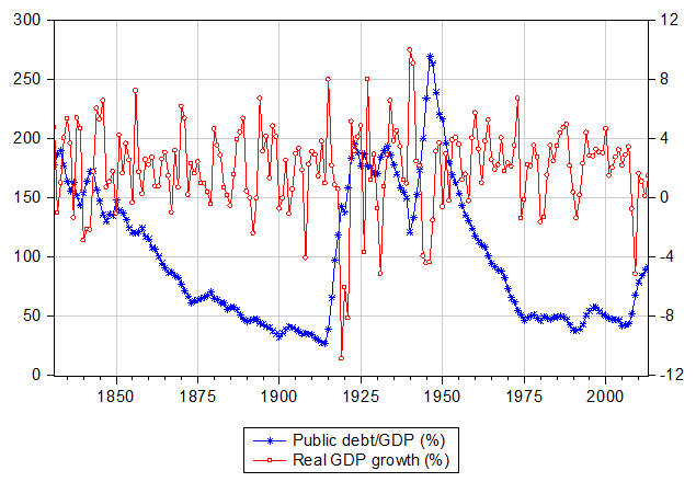
Data sources: International Monetary Fund (IMF) historical database, Bank of England three centuries of data and website of Professor Carmen Reinhart.
Note: Real GDP growth is constructed as 100*(y_t-y_t-1)/y_t-1  where y_t is the level of real GDP. Real GDP growth is stationary series using conventional Augmented Dickey Fuller (ADF) tests: Assuming a constant and 4 lags (based on the Akaike Information Criterion), the ADF test statistic for real GDP growth is equal to -6.24 (p-value=0.00). The evidence of Debt/GDP stationarity is less clear. Assuming a constant and 4 lags (based on the Akaike Information Criterion), the ADF test statistic for debt/GDP is equal to -2.78 (p-value=0.06). p-values are the MacKinnon (1996) one-sided p-values. On the other hand, allowing for a break in the intercept, a Zivot-Andrews (1992) unit root test (using 3 lags) delivers stationarity for debt/GDP as the t-statistic is equal to -5.16 (the 5% critical value=-4.80) with a break identified in 1915.

As I noted in my previous post, the two variables have a mild negative correlation (equal to -0.11). However, a negative correlation does not establish causality. How did I identify if there is any significant relationship between the two variables? I treated both variables as endogenous within a Vector Autoregressive (VAR) model which also controls for the endogenous effects of CPI inflation and the policy interest rate (as a proxy for UK’s cost of borrowing). The VAR model was estimated assuming a lag length of two lags based on the Akaike Information Criterion (AIC).

I now augment my model to include the exogenous effects of World War I and World War II (treating these as two separate exogenous dummy variables) and (again) choosing a lag length of two lags (based on the Akaike Information Criterion). My model distinguishes between a “high” and a “normal” (or lower) growth regime. Both regimes are endogenously determined by the data (we, econometricians, call this a regime switching Threshold VAR model; for those interested in the econometrics, the Threshold VAR model chose a delay parameter of 1 based on Tsay’s (1998) test). I “run” the model using the 1831-2013 dataset and observe how positive shocks (“impulse responses”) to public debt impact on GDP growth. For those interested in the econometrics, I use a Cholesky decomposition with the following order in the VAR: [cpi inflation, real GDP growth, interest rate, debt/GDP]’. Ordering inflation and output before the interest rate is standard in the literature but I will return to this issue below. The main results are summarised as follows:

1. As in my previous post, and allowing for the exogenous world war effects, the model results (entirely driven by the data) distinguish between (i) a high GDP growth regime (equal to 2.98% per annum or higher) and (ii) a normal (or lower) growth regime (when annual real GDP growth drops below 2.98%). Both in the high growth regime and in the low growth regime, a positive public debt shock has a negative impact on UK growth within a 4-year horizon (see Figure 2 and Figure 3 below); the impact is “much less” significant in the high growth regime. Figure 2 plots the median response of real GDP growth to a public debt/GDP (equal to one standard deviation) shock when the economy is “booming”. Figure 3 plots the median response of real GDP growth to a public debt/GDP (equal to one standard deviation) shock when the economy is in the normal and/low growth regime. Whatever the regime, a higher debt/GDP ratio does drag real GDP growth down. (Note to readers: action is taken in period 0 (now) and we look at its impact within a 4-year horizon). In what follows, I report further robustness checks. All of these checks use the world war dummies as exogenous variables.
2. The policy rate, despite being a policy “instrument”, is definitely not a good proxy of UK’s cost of borrowing. To account for this, I rerun the model using (instead) the 10-year UK yield. Again, I allow for the exogenous effect of the two world wars. The reader will notice (see Figure 4 and Figure 5) that results remain robust to this alternative specification.
3. My Cholesky “structure” treats debt/GDP as the most endogenous variable. As an alternative, I used generalized impulse responses (see Pesaran and Shin) that do not require orthogonalization of shocks and are invariant to the ordering of the variables in the VAR. Figure 6 and Figure 7 confirm that debt/GDP drags real growth down (my model uses the 10-year yield rather than the policy rate).
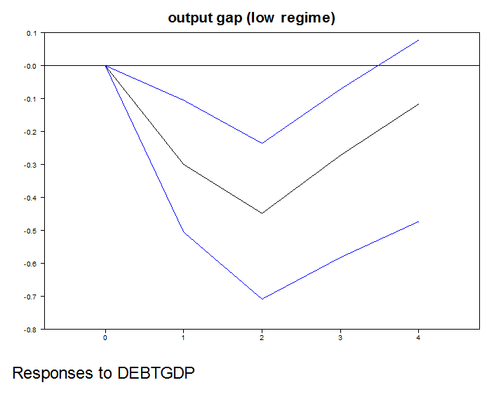
4. Rather than looking at the impact of debt/GDP on real GDP growth, I look at the impact of debt/GDP on the output gap (output relative to potential). The output gap is plotted in Figure 8. Of course, the output gap is notoriously difficult to estimate. What I do, for this post, is the following: For 1831-1954, I pool together information from different filters. In particular, I proxy the output gap by the median of (i) output gap using a Hodrick-Prescott trend, (ii) output gap using a cubic trend and (iii) output gap using the full sample asymmetric Christiano-Fitzgerald (2003) filter. From 1955 onwards, I use the output gap measure of the Office for Budget Responsibility (OBR). My empirical VAR model uses the 10-year yield (rather than the policy rate). The Threshold VAR (based on two lags) identifies a low output gap regime (output gap below -1.30%) and a “(quasi-normal” (or better) output gap regime (output gap above -1.30%). Figure 9 and Figure 10 confirm that debt/GDP depresses the output gap (the impact is statistically significant in the low output gap regime). These results are based on the Cholesky decomposition structure mentioned above (rather than the Pesaran and Shin approach).
5. In all estimations, I used CPI inflation rather than inflation based on the GDP deflator. My critics at www.pieria.co.uk argued that “CPI can’t really be regarded as an endogenous variable, since it includes items within the basket that are vulnerable to exogenous shocks. It would have been better to have used core inflation or the GDP deflator.”  Indeed, I would have loved to use core inflation (if this data were available from… 1831 but I think they are not).  On the other hand, I do not think that use of the GDP deflator would have made any substantial difference. And one other thing: CPI not endogenous? Really? Please mention this to the Monetary Policy Committee (MPC) members who are targeting CPI inflation.
6. Last (but not least) I could have rerun the model from 1946 (or 1950) onwards. I do not want to do this as in this case I have very few data (between 1946-2013) available for meaningful estimation of the Threshold VAR.

All of the above suggest that debt/GDP drags real GDP growth down. In any case, I hope to produce a full working paper related to this issue and to the issue of the stronger depressing impact of an interest rate hike on GDP growth in “good times”; see also on this the work of University of Manchester colleagues, Sensier, Osborn and Ocal.

Figure 2: Response of GDP growth (Left Hand Side Axis) to DEBT/GDP shock within a 4-year horizon (Horizontal axis). High growth regime.

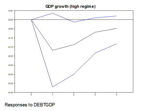
Figure 3: Response of GDP growth (Left Hand Side Axis) to DEBT/GDP shock within a 4-year horizon (Horizontal axis). Normal (and/or low) growth regime. 

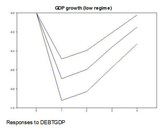
Figure 4: Response of GDP growth (Left Hand Side Axis) to DEBT/GDP shock within a 4-year horizon (Horizontal axis). High growth regime (results based on 10-year UK yield).

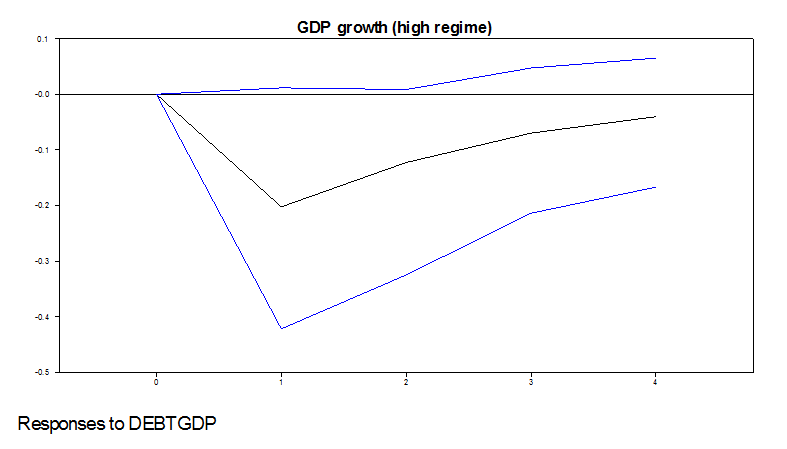
Figure 5: Response of GDP growth (Left Hand Side Axis) to DEBT/GDP shock within a 4-year horizon (Horizontal axis). Normal (and/or low) growth regime (results based on 10-year UK yield).

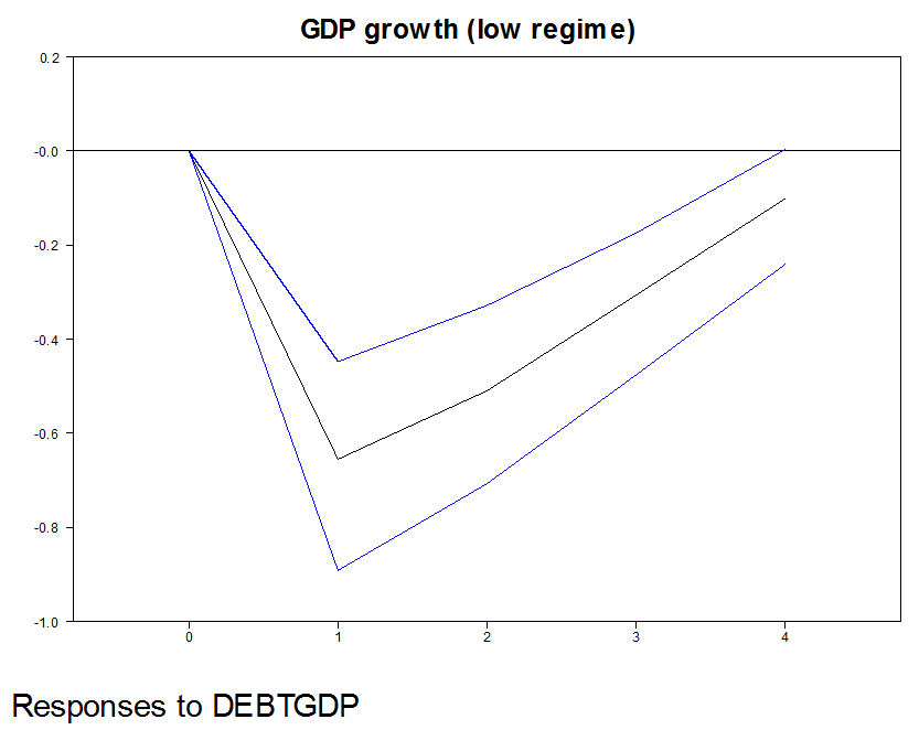
Figure 6: Response of GDP growth (Left Hand Side Axis) to DEBT/GDP shock within a 4-year horizon (Horizontal axis). High growth regime (results based on 10-year UK yield). Based on the Pesaran and Shin (1998) generalized impulse responses.

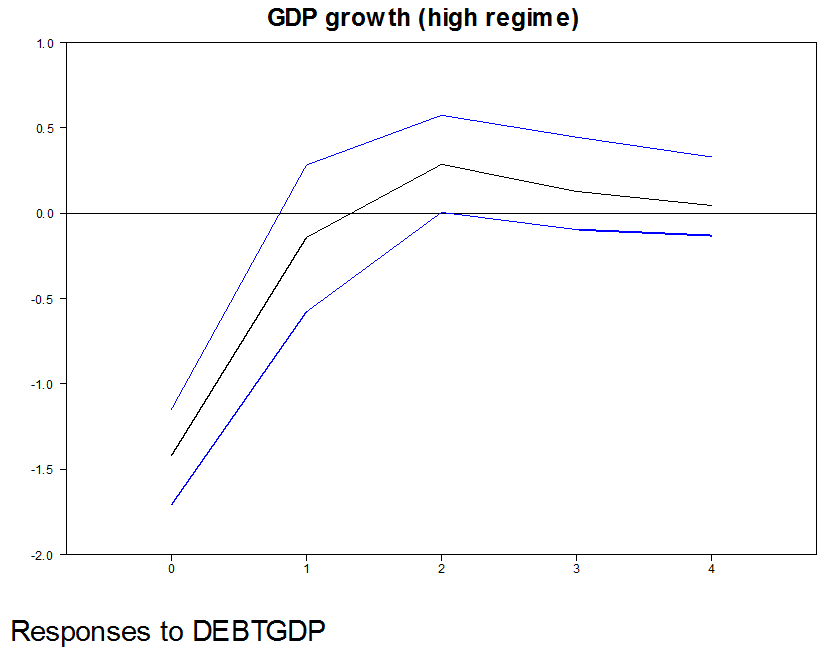
Figure 7: Response of GDP growth (Left Hand Side Axis) to DEBT/GDP shock within a 4-year horizon (Horizontal axis). Normal (and/or low) growth regime (results based on 10-year UK yield). Based on the Pesaran and Shin (1998) generalized impulse responses.

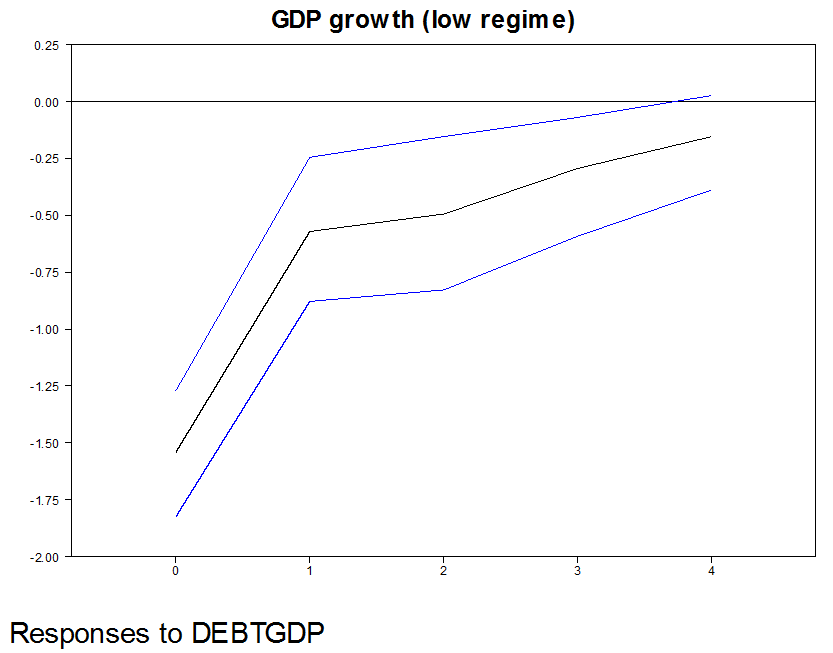
Figure 8: UK output gap (%, output relative to potential) 1831-2013

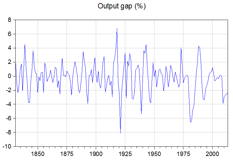
Notes: For 1831-1954, the output gap is the median of (i) output gap using a Hodrick-Prescott trend, (ii) output gap using a cubic trend and (iii) output gap using the full sample asymmetric Christiano-Fitzgerald (2003) filter. From 1955 onwards, I use the output gap measure of the Office for Budget Responsibility (OBR).

Figure 9: Response of output gap (Left Hand Side Axis) to DEBT/GDP shock within a 4-year horizon (Horizontal axis). “Quasi-normal” (or better) output gap regime (results based on 10-year UK yield).

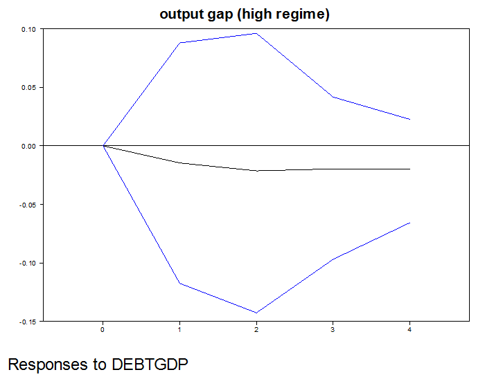
Figure 10: Response of output gap (Left Hand Side Axis) to DEBT/GDP shock within a 4-year horizon (Horizontal axis). Low output gap regime (results based on 10-year UK yield).

Note:  This article gives the views of the author, and not the position of the British Politics and Policy blog, nor of the London School of Economics. Please read our comments policy before posting. 

About the Author

Costas Milas is Professor of Finance at the University of Liverpool Management School. Email: costas.milas@liverpool.ac.uk