


 Each month, the team from electionforecast.co.uk compare new constituency polls as they are released to their estimates of what polls would show in those constituencies. This allows for an assessment of the accuracy of their modelling approach. More information about the overall model can be found here. The results presented in this post use the Scotland constituency polls released by Lord Ashcroft on 3 February 2015.
As we have said previously, estimating the support in each constituency is essential for accurate election forecasts. Constituency polls allow us to look beyond national level support for the parties, and help with understanding how votes might translate into seats on May 7th.
In addition to providing our model with this important information, they also offer an opportunity to evaluate how the model is performing. As we did for the release of Lord Ashcroft’s November and December polls, in this post we compare the Scotland constituency polls released on 3 February to our estimates of what such polls would show from earlier that day. This is a test of our model’s ability to accurately predict what polls should show in constituencies where there has not yet been a poll.
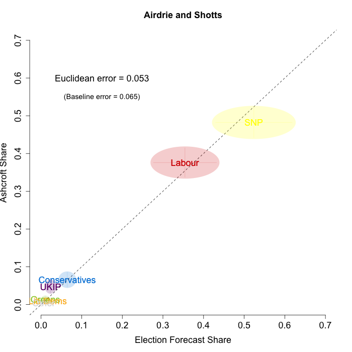
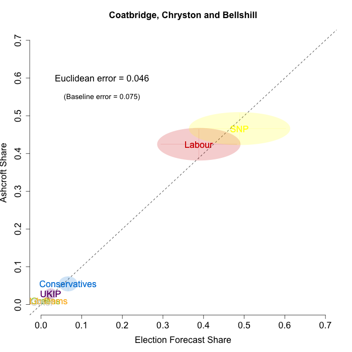
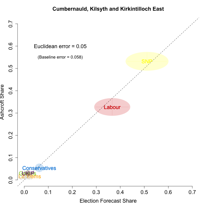
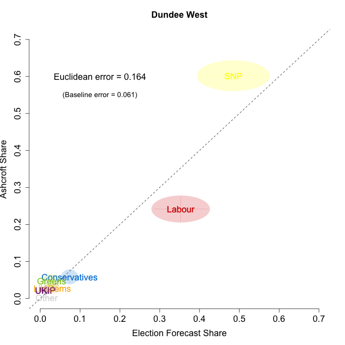
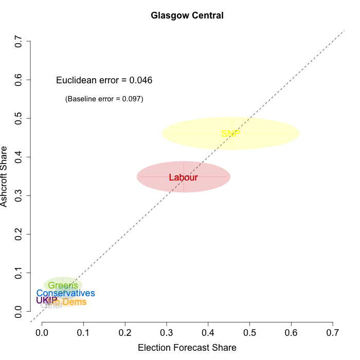
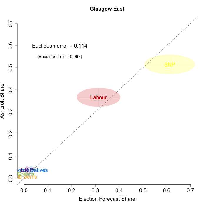
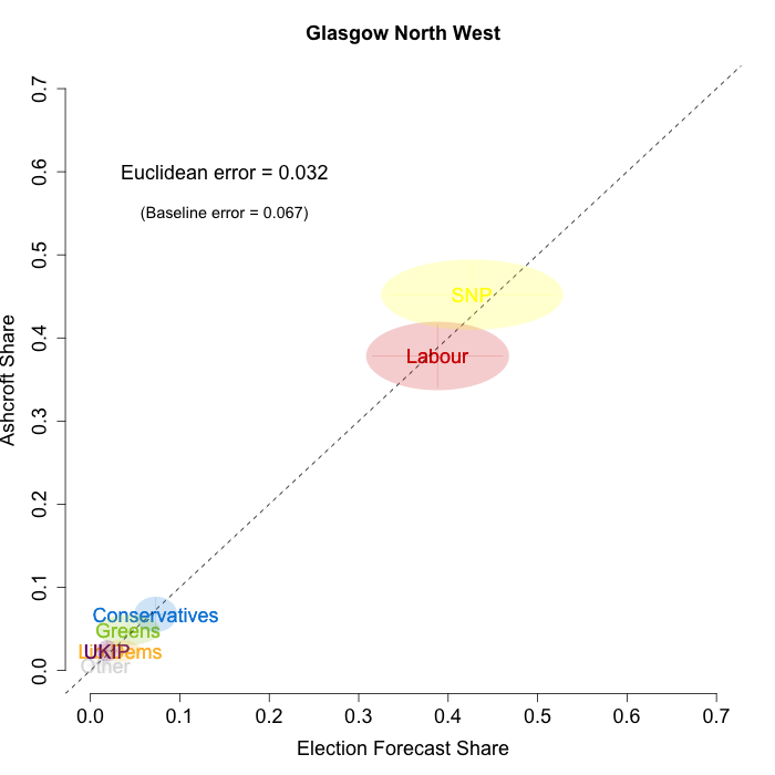
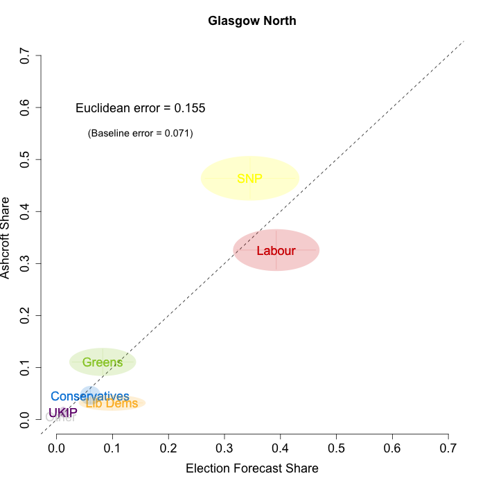
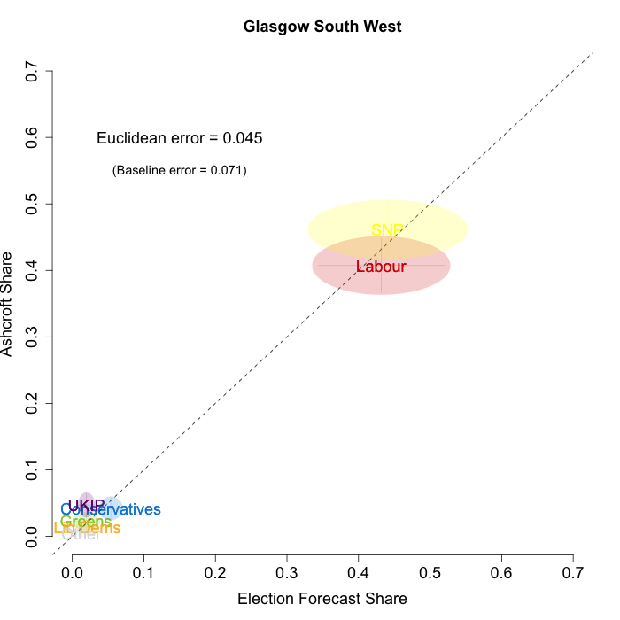
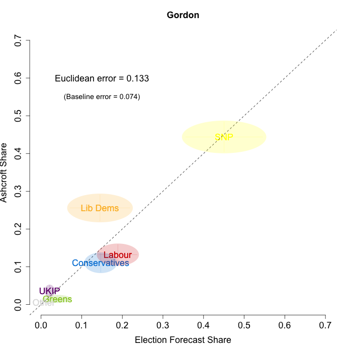
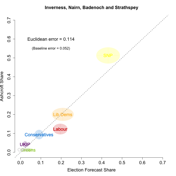
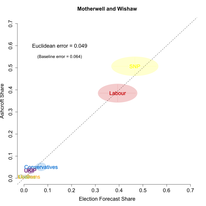
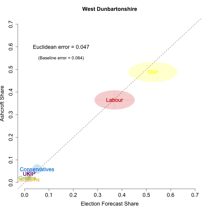
The plots below show that in most of the 16 Scottish constituencies polled by Lord Ashcroft, we are accurately recovering the current state of play. We plot our estimates from 3 February for these constituencies on the x-axis and the Ashcroft estimates on the y-axis.
Both the polls and our estimates include uncertainty; in the figures below we break these results out by constituency and plot ellipses capturing the joint margin of error around each point. Whenever these ellipses cross the dashed 45-degree line, we can say that our predicted vote share range for a given party, in a given constituency, coincides with the range implied by Lord Ashcroft’s polls.
Navigating through each constituency shows that despite the lack of previous constituency polling in Scotland, we had good estimates of vote intention in the polled constituencies. We have one major miss (in Glasgow North where we had Labour ahead and Ashcroft found SNP ahead) and one moderate miss (in Paisley and Renfrewshrew South, where we had Labour and SNP tied and Ashcroft found SNP ahead) but in all the other constituencies we had the key facts right.
- Airdrie and Shotts
- Coatbridge, Chryston and Bellshill
- Cumbernauld, Kilsyth and Kirkintilloch East
- Dundee West
- Glasgow Central
- Glasgow East
- Glasgow North East
- Glasgow North West
- Glasgow North
- Glasgow South West
- Glasgow South
- Gordon
- Inverness, Nairn, Badenoch and Strathspey
- Motherwell and Wishaw
- Paisley and Renfrewshire South
- West Dunbartonshire
But this is an impressionistic accounting; how can we make this evaluation more precise? There are two kinds of standards against which we could assess the performance of our estimates at predicting the Ashcroft polls.
The first way to assess our estimates of voting intention in the constituencies is against the level of uncertainty that we were claiming for those estimates. Each of our estimates comes with a degree of uncertainty, as does each of the Ashcroft polls. These are depicted in the ovals around each point in the plots. Are these the correct size, or were we falsely confident in our predictions of where support stood in these Scottish constituencies?
To assess the overall magnitude of our errors across all parties in each constituency, we compute a Euclidean distance between our estimates and Ashcroft’s polls. We thank the mysterious poster “Unicorn” on ukpollingreport.co.uk for suggesting the Euclidean distance measure. This is a measure of the total distance between two sets of party vote shares in a constituency. We do not expect these to be zero because of uncertainty in our estimates and sampling error in Ashcroft’s polls, so we also calculate the expected Euclidean distance given our uncertainty estimates and the uncertainty estimates associated with a poll of the size that Ashcroft reports. We can calculate both the actual difference between our estimates and Ashcroft’s poll and the expected magnitude of that distance in each constituency. These are shown on the plots for each constituency. Averaging across all constituencies, the mean distance between our estimates and Ashcroft’s polls 7.7 percentage points. Given the size of the polls and the uncertainty we were calculating for our estimates, we would have expected it to be 6.8 percentage points. So we were a little overconfident in our estimates, but only a little. Overall, our predictions were very nearly as good as they claimed to be.
But was that actually any better than a simpler approach like applying uniform swing? This is the second way we can assess our estimates. Here we again use the Euclidean distance, but comparing the distances between our estimates and Ashcroft’s polls to the distances between other predictions we could have made and those polls. Obviously a Great Britain uniform swing model will perform horribly because SNPs swing is entirely concentrated in Scotland, so we will focus on Scotland-specific uniform swing models. Do we do better than uniform swing? Put differently, are we successful at measuring the ways in which the Scottish swing is not uniform?
There is no single right way to calculate a Scotland-only swing for comparison, but here are three that give uniform swing a good chance to do as well as our model. First, we might calculate the Scotland swing by taking our poll estimates for all of Scotland, calculate the average swing implied by those, and then apply that average swing to all 2010 constituency-level results. If we do this, the mean Euclidean distance is 13.7 percentage points, versus 7.7 for our estimates. This approach does poorly because the swing across Scotland is not uniform. The Ashcroft polls were targeted at the constituencies likely to see the greatest swings: traditional Labour strongholds with high Yes votes.
To make a uniform swing approach the performance of our estimates, we need to further reduce the set of constituencies we apply the uniform swing to: not all of Great Britain, not even all of Scotland, but just the polled constituencies. If we calculate the average swing from our poll estimates using only the constituencies that Ashcroft polled, and then apply that average swing to all 2010 constituency-level results, the mean Euclidean distance is 9.3 percentage points. So we are doing better than a uniform swing, even just applied among the polled constituencies. We can take this further, and calculate the average swing across the Ashcroft constituency polling itself, and use that to apply a uniform swing to the polled constituencies. This is an extremely tough comparison for our predictions, because it actually uses the Ashcroft constituency polls, ensuring that it applies the best possible uniform swing for predicting those polls. With this method, the mean Euclidean distance is 8.2 percentage points. Thus, even knowing exactly the average swing in the Ashcroft polls, and applying that swing uniformly across the polled constituencies, you would be less successful at predicting the constituency-level results in those polls than by taking our estimates from before the polls were released.
Overall, we remain pleased at how well our model seems to be performing at predicting Ashcroft constituency polls before they are released, which gives us additional confidence looking forward to the election. With the new Scotland constituency polls, one of the largest remaining sources of uncertainty about the election has been substantially reduced. Still, there are three months between now and the election, and significant changes may still occur, as they have historically. Our model aims to capture this in the uncertainty that it reports about the election results, and we will continue to update as new data arrives over the coming months.
 Jack Blumenau is a PhD candidate in Government at the London School of Economics.
 Chris Hanretty is a Reader in Politics at the University of East Anglia.
 Benjamin Lauderdale is an Associate Professor in Methodology at the London School of Economics.
 Nick Vivyan is a Lecturer in Quantitative Social Research at the Durham University.







Thanks for the info. I’m following the use of your method with considerable interest. I’ll be interested to see how it compares with the techniques previously used for, for example, extrapolating exit polls into votes.